EOQ (Economic Order Quantity)
4 min read
By
TranZact Solutions Team
· Published


Economic Order Quantity (EOQ) is the order size that minimizes combined ordering and holding cost. It is calculated from annual demand, cost per order, and holding cost per unit. The textbook formula assumes steady, predictable demand, which is exactly why it needs adjustment for most Indian manufacturing SMEs with seasonal or lead-time-variable supply.
Ordering too much ties up cash in stock sitting on a shelf. Ordering too little means more frequent orders and a higher chance of running short. EOQ is the formula built to find the middle.
What Is EOQ?
Economic Order Quantity is the order quantity that minimizes total inventory cost: ordering cost plus holding cost. Ordering cost is what it costs to place and process an order. Holding cost is what it costs to store that inventory until it’s used.
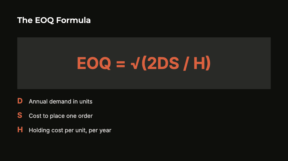
The classic EOQ formula is the square root of (2 × annual demand × ordering cost ÷ holding cost per unit per year). As order size goes up, ordering cost per unit falls but holding cost rises. EOQ finds the quantity where the two curves cross.
EOQ was built for a world of stable demand and fixed lead times. It works cleanly for raw material with steady, predictable consumption. It breaks down fast for seasonal items, new products with no demand history, or vendors with inconsistent lead times.
EOQ vs Just-In-Time Ordering
Order size: EOQ calculates one fixed optimal quantity per order; JIT uses small, frequent orders sized to near-term need.
Assumption: EOQ assumes stable demand and lead time; JIT assumes reliable, fast vendor delivery so large buffer orders aren’t needed at all.
Cash impact: EOQ still ties up cash in a calculated buffer; JIT minimizes cash tied up by ordering closer to actual consumption.
Risk: EOQ is more forgiving of a single late delivery since it carries more stock per order. JIT is more exposed to vendor delays since buffer stock is minimal.
Manufacturer relevance: EOQ suits stable, high-volume raw material with reliable vendors; JIT suits high-value or fast-moving materials where vendor lead times are dependable. Many manufacturers run a mix of both.
Want to see your real stock and purchase numbers before you set order sizes?
How to Calculate EOQ
Working out EOQ comes down to three inputs and one formula:
Annual demand (D). Total units consumed over a year, based on actual historical usage, not a rough guess.
Ordering cost (S). The cost to place and process a single purchase order (admin time, follow-up, receiving effort). It is not just the item price.
Holding cost per unit (H). The annual cost to store one unit, covering warehousing, insurance, capital tied up, and shrinkage risk.
Apply the formula. EOQ equals the square root of (2 times D times S divided by H). A worked example: annual demand of 12,000 units, ordering cost of ₹500 and holding cost of ₹20 per unit. That gives an EOQ of about 775 units per order.
Worked example: EOQ in five steps
Annual demand D: 12,000 units
Cost per order S: ₹500
Holding cost H: ₹20 per unit
2DS ÷ H = 6,00,000
Square root: about 775 units per order
Where the EOQ Formula Breaks Down
The textbook formula assumes conditions that rarely hold in a real Indian manufacturing SME:
Assumes constant, predictable demand. Seasonal products or new SKUs with no usage history don’t have a reliable demand number to plug into the formula.
Assumes a fixed, reliable lead time. A vendor with inconsistent delivery dates makes any fixed order-size formula risky without a safety-stock buffer added on top.
Ignores quantity discounts. Many suppliers offer per-unit price breaks at higher order volumes that the basic formula doesn’t account for at all.
Treats holding cost as a flat, known number. Most SMEs don’t actually calculate their true holding cost (warehousing, capital, shrinkage). So the formula runs on a guessed input.
Used once and never recalculated. Demand, costs, and vendor terms all shift; an EOQ calculated a year ago is often quietly wrong today.
Do you know your real annual demand and holding cost per SKU, or is your order quantity still based on habit?
How TranZact Supports Order Quantity Decisions
TranZact shows what is actually happening with your stock right now, so order quantities start from current data, not a guess.
The inventory module covers stock in, issue, bin card, multi-store, reorder and AI stock alerts. Inventory ageing and valuation come with the Scale and Dominate plans.
For purchase planning, the MRP engine runs through your orders and BOMs, then tells you what to buy and when. Planning (MRP + Indent) is on Scale and Dominate.
It doesn’t replace the judgment call on vendor discounts or seasonal buffers. What it removes is calculating EOQ off stale or guessed demand numbers in the first place.
If your order sizes still come from habit, start from real numbers. See how TranZact handles stock and purchase planning for a manufacturer like you.